Note
Click here to download the full example code
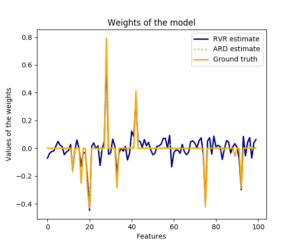
Comparison of relevance vector regression and ARDRegression
print(__doc__)

import matplotlib.pyplot as plt
import numpy as np
from scipy import stats
from sklearn.linear_model import ARDRegression
from sklearn_rvm import EMRVR

# #############################################################################
# Generating simulated data with Gaussian weights

# Parameters of the example
np.random.seed(0)

n_samples, n_features = 100, 100

# Create Gaussian data
X = np.random.randn(n_samples, n_features)
# Create weights with a precision lambda_ of 4.
lambda_ = 4.
w = np.zeros(n_features)
# Only keep 10 weights of interest
relevant_features = np.random.randint(0, n_features, 10)
for i in relevant_features:
    w[i] = stats.norm.rvs(loc=0, scale=1. / np.sqrt(lambda_))
# Create noise with a precision alpha of 50.
alpha_ = 50.
noise = stats.norm.rvs(loc=0, scale=1. / np.sqrt(alpha_), size=n_samples)
# Create the target
y = np.dot(X, w) + noise

# #############################################################################
# Fit the ARD Regression
clf = ARDRegression(compute_score=True)
clf.fit(X, y)

rvr = EMRVR(kernel="linear")
rvr.fit(X, y)

# #############################################################################
# Plot the true weights, the estimated weights, the histogram of the
# weights, and predictions with standard deviations
plt.figure(figsize=(6, 5))
plt.title("Weights of the model")
plt.plot(rvr.coef_, color="darkblue", linestyle="-", linewidth=2, label="RVR estimate")
plt.plot(clf.coef_, color="yellowgreen", linestyle=":", linewidth=2, label="ARD estimate")
plt.plot(w, color="orange", linestyle="-", linewidth=2, label="Ground truth")
plt.xlabel("Features")
plt.ylabel("Values of the weights")
plt.legend(loc=1)
plt.show()
Total running time of the script: ( 0 minutes 17.338 seconds)